
14 Multi-Level Modelling
Crossfit Gyms is growing - they started the year with 5 locations and have more than doubled in size in the last five months. Additionally, Crossfit Gyms has secured funding to open 100 more gyms over the next year. Their key recruitment mechanism is to offer free trial memberships that last a calendar month, but management is unsure how to measure the success of this trial. Additionally, some gyms have been randomly chosen to increase the stretching, called “Yoga Stretch”, done during these trial classes. Crossfit Gyms is unsure whether this has helped convert trial customers into memberships. The theory is that new members, typically less athletic than current clients, benefit from the additional stretching and are more likely to enjoy the additional stretch time.
In this chapter, our task is to help Crossfit Gyms understand the effect of its trial membership program and whether additional stretching leads to better conversion of free-trial customers into paying members. As we go through this example, we will explore three different ways to model the conversion rates at this franchise’s gyms:
This is a long chapter, consider reading one section per sitting. I find walking away, sleeping, and then returning from challenging or frustrating code to be more efficient than spending an equivalent amount of time staring at the same problem. Fresh eyes will make you smarter.
Modelling Only Franchise-Level Conversion Rates: This modelling method, known as complete pooling, aggregates all the data for all the gyms. It will model two conversion rates for the entire franchise - one with yoga stretching and one without. All gyms are considered interchangeable when doing this as they each have identical data generating processes.
Modelling Only Gym-Level Conversion Rates: This method, known as no pooling, will treat each gym individually with the underlying assumption that the two conversion rates (with and without yoga) at one gym are completely independent of conversion rates at every other gym. Since there are 12 gyms in the dataset, 24 conversion rates will be modelled. This model assumes knowing one gym’s conversion rate will NOT be useful for predicting another gym’s conversion rate.
Modelling Franchise-Level and Gym-Level Conversion Simultaneously: Under this method, known as partial pooling, we assume each gym’s two conversion rates have both a unique component (like the no pooling case) as well as a component that is dictated by company-wide policies (like the complete pooling case). This model estimates the conversion rate for each gym as well as the overall conversion rate for all gyms, while accounting for the variability and uncertainty in the data.
14.1 The Gym Data
Let’s explore the Crossfit Gyms data. Here, we load the data into pandas and present the first 10 rows.
import pandas as pd
url = "https://raw.githubusercontent.com/flyaflya/persuasive/main/gym.csv"
gymDF = pd.read_csv(url)
gymDF.head(10)
gymID timePeriod nTrialCustomers nSigned yogaStretch
0 1 1 32 7 0
1 2 1 56 4 0
2 3 1 42 1 0
3 4 1 58 9 0
4 5 1 84 44 0
5 1 2 38 14 0
6 2 2 68 7 0
7 3 2 42 3 0
8 4 2 64 13 0
9 5 2 72 33 0When thinking about visualizing this dataset, we need to understand what each row represents; in particular we observe that each row is an observation of a particular time period at a particular gym. Wondering how many observations exist for each gym, we do a quick split-apply-combine workflow:
(  ## open parenthesis to start readable code
    gymDF
    .groupby("gymID") ## split into group of df's, one for each gym
    .size() ## count # of rows in each and recombine into single df
) ## close parenthesis finishes the "method chaining"
gymID
1 5
2 5
3 5
4 5
5 5
6 4
7 4
8 4
9 3
10 2
11 1
12 1
dtype: int64to discover that we have twelve unique gyms; the first 5 gyms give us five months of data each, while the next seven have less data (ranging from one to four free-trial months).
Since the small gymdDF data frame consists of only five variables (i.e. columns), I am confident that I can map all five to visual aesthetics and show all the data using one plot command. After several iterations of plots (excluded here), here is the mapping I have chosen:
\[ \begin{aligned} \textrm{Chosen } Geometry &= interval &(\mathtt{ax.barh})\\ \hline\\ \textrm{Gym} &\rightarrow \textrm{facet} &(\mathtt{axs[0,0] \ldots axs[3,4]})\\ \textrm{Time Period} &\rightarrow \textrm{horizontal postion } &(\mathtt{width})\\ \textrm{\# of Trial Customers} &\rightarrow \textrm{vertical postion} &(\mathtt{y})\\ \textrm{\# of Customers Converted To Members} &\rightarrow \textrm{vertical postion} &(\mathtt{y})\\ \textrm{Yoga Stretch Indicator} &\rightarrow \textrm{color } &(\mathtt{color}) \end{aligned} \]
Note that I can map two columns in the dataframe to the y-position because they share the same units of measure. Both trial participants and the number of those participants converted to gym members are just counts of people.
While I find the conceptual mapping above somewhat easy to specify, it is more involved to get matplotlib to make the right plot for you. Breaking a complex coding challenge like this into smaller, manageable tasks can help to make it less daunting. As a source of inspiration, we can look to the words of Dr. Martin Luther King Jr., who famously said:
“If you can’t fly, then run. If you can’t run, then walk. If you can’t walk, then crawl. But whatever you do, you have to keep moving forward.” - Dr. Martin Luther King Jr.
Crawling towards an initial plot, I make my goal much smaller. Namely, get the plot working for one gym, say Gym #1. Here is the code to do that:
import matplotlib.pyplot as plt

# get just gym 1
gymGroupedDF = gymDF.groupby("gymID")
grpDF = gymGroupedDF.get_group(1)

fig, ax = plt.subplots(figsize = [5,3.5], layout = "constrained")

# labels to help our audience
fig.suptitle("Converting Free Trials to Paying Members")
ax.set_title("Gym 1")
ax.set_xlabel("Time Period")
ax.set_ylabel("# of Customers")

# create boolean masks to filter the rows by yogaStretch value
has_yoga = grpDF["yogaStretch"] == 1
no_yoga = grpDF["yogaStretch"] == 0

# plot the bars for each group separately
yogaTrial = ax.bar(
  grpDF.loc[has_yoga, "timePeriod"],
  grpDF.loc[has_yoga, "nTrialCustomers"],
  color = "thistle",
  label = "Yoga Trial"
)

yogaMember = ax.bar(
  grpDF.loc[has_yoga, "timePeriod"],
  grpDF.loc[has_yoga, "nSigned"],
  color = "darkorchid",
  label = "Became \na Member"
)

noYogaTrial = ax.bar(
  grpDF.loc[no_yoga, "timePeriod"],
  grpDF.loc[no_yoga, "nTrialCustomers"],
  color = "powderblue",
  label = "No Yoga Trial"
)

noYogaMember = ax.bar(
  grpDF.loc[no_yoga, "timePeriod"],
  grpDF.loc[no_yoga, "nSigned"],
  color = "cadetblue",
  label = "Became \na Member"
)

ax.legend(
  handles = [yogaTrial, yogaMember, noYogaTrial, noYogaMember],
  bbox_to_anchor=(1, 0.5), loc='center left', ncol = 1
)

plt.show()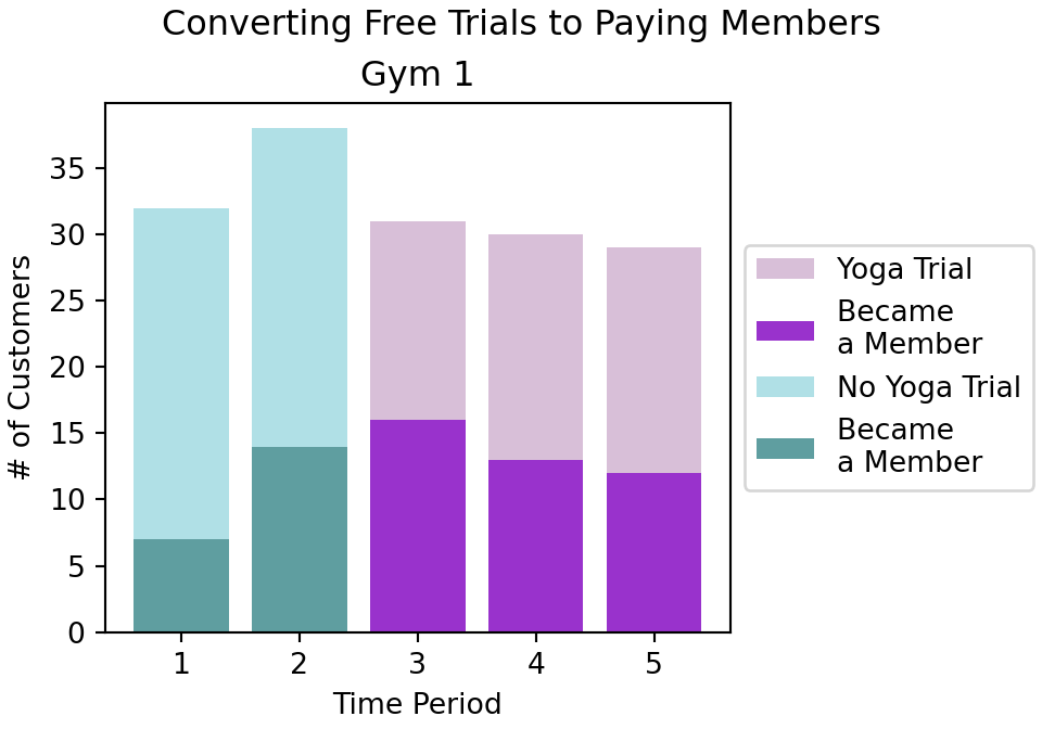
Figure 14.1 reveals that Gym #1 has had two time periods without yoga and two time periods with yoga. It seems a larger percentage of trial members converted when using yoga as the darker fill is a larger percentage of the bars.
Let’s see what we can learn from a facet plot showing all the gyms:
import matplotlib.pyplot as plt
import matplotlib.patches as mpatches

# compute number of gyms for laying out figure
numGyms = gymDF['gymID'].nunique()

# create enough subplots (assume four columns)
num_cols = 4
num_rows = (numGyms - 1) // num_cols + 1  ## // is floor division

# create figure
fig, axes = plt.subplots(
  nrows=num_rows,
  ncols=num_cols,
  sharex = True,
  sharey = True,
  figsize=(12, 2.5*num_rows),
  layout = "constrained")

fig.suptitle("Trial Memberships By Gym With Darker Fill Used To Show Conversions to Paying Customers")

# iterate through gyms creating bar plots left to right with four columns
for i, (gymID, grpDF) in enumerate(gymGroupedDF):
    row = i // num_cols
    col = i % num_cols
    ax = axes[row, col]
    ax.set_title(f'Gym {gymID}')
    if row == num_rows:
        ax.set_xlabel("Time Period")
    if col == 0:
        ax.set_ylabel("# of Customers")
    # create boolean masks to filter the rows by yogaStretch value
    has_yoga = grpDF["yogaStretch"] == 1
    no_yoga = grpDF["yogaStretch"] == 0

    ## same code as above, just using gymDF
    # create bars for yoga and non-yoga trials
    yogaTrial2 = ax.bar(
        grpDF.loc[has_yoga, 'timePeriod'],
        grpDF.loc[has_yoga, 'nTrialCustomers'],
        color='thistle',
        label='Yoga Stretch Trial'
    )
    noYogaTrial = ax.bar(
        grpDF.loc[no_yoga, 'timePeriod'],
        grpDF.loc[no_yoga, 'nTrialCustomers'],
        color='powderblue',
        label='No Yoga Trial'
    )

    # create bars for yoga and non-yoga paying members
    ax.bar(
        grpDF.loc[has_yoga, 'timePeriod'],
        grpDF.loc[has_yoga, 'nSigned'],
        color='darkorchid'
    )
    ax.bar(
        grpDF.loc[no_yoga, 'timePeriod'],
        grpDF.loc[no_yoga, 'nSigned'],
        color='cadetblue'
    )

# use patch objects for the legend
yogaTrialPatch = mpatches.Patch(color='thistle', label='Yoga Stretch Trial')
noYogaTrialPatch = mpatches.Patch(color='powderblue', label='No Yoga Trial')
# place legend in bottom-right box where there is white space
ax = axes[2, 3]
ax.legend(
handles = [yogaTrialPatch, noYogaTrialPatch],
bbox_to_anchor=(0.02, 0.7), loc='center left', ncol = 1
)
plt.show()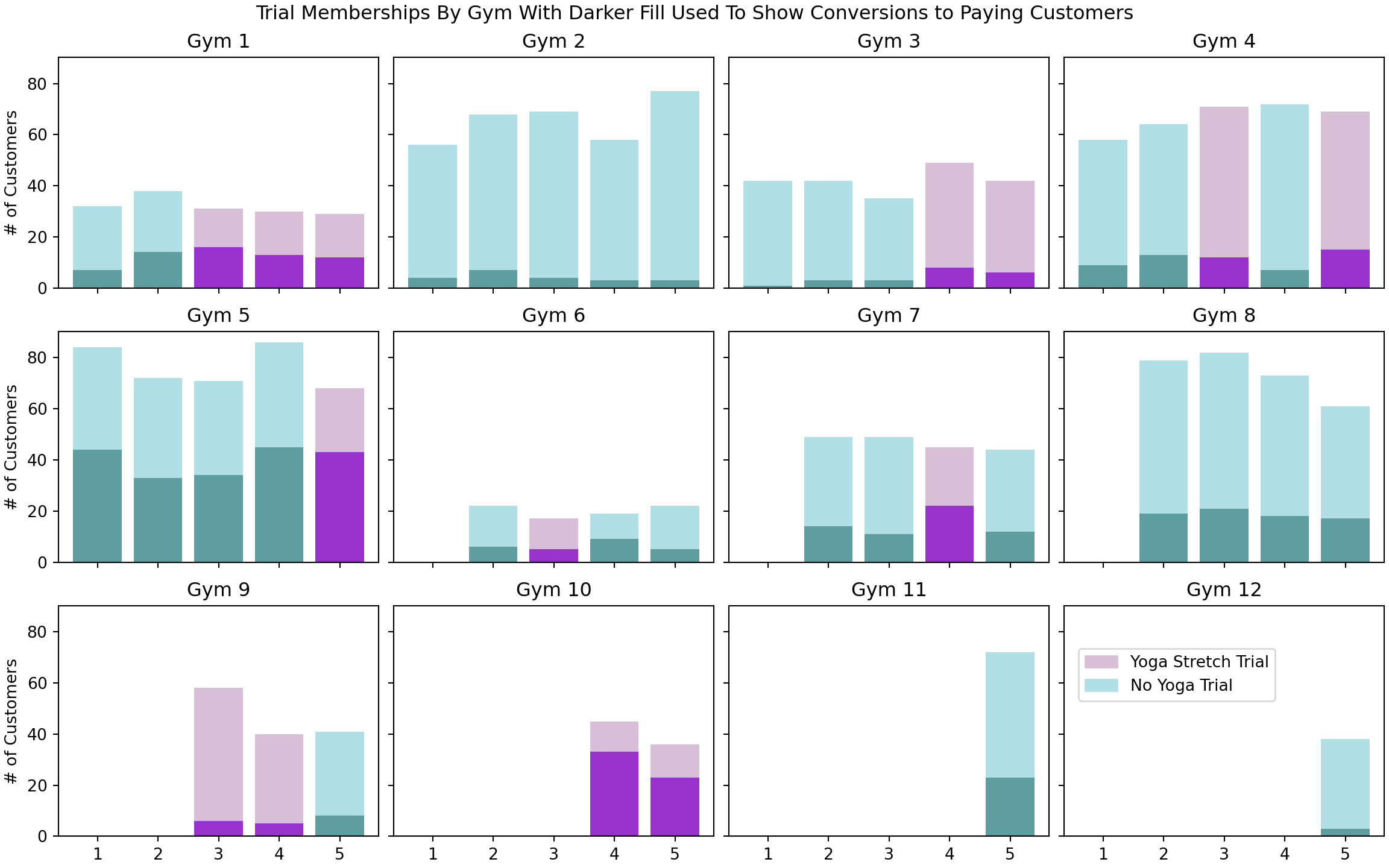
You can see from Figure 14.2 that the recruitment rate at each gym, represented by the proportion of dark fill to lighter fill, seems pretty consistent. However, there is apparent high variability across gyms. For example, Gym 2 seems to be a consistently poor performer while Gym 5 is somehow able to consistently make more conversions from free trials to paying memberships.
Talking to the managers of these gyms to understand the differences in performance should be high on your to-do list, but for now (and because we do not have access to these managers), we will stick with the data that is available.
In terms of providing insight as to recruitment rates and the effect of extra yoga stretching (indicated by fill color), the visualization can only go so far. Yes, we can say Gym 5 outperforms Gym 2, but with only five months of data, how can we quantify our uncertainty about the differences? Additionally, yoga stretching seems to lead to better conversion rates, but how confident should we be given the seemingly small amounts of data\(^{**}\)?
** Actually, the data size is not as small as you might think. While only 44 combinations of gym and time periods are observed, Crossfit Gyms has seen over 2,000 customers participate in a free trial.
14.2 Complete Pooling
The complete pooling model is a slight misnomer as we have two distinct groups of observations. One group is with traditional stretching and the other yoga stretching. All gyms in the entire franchise behave the same. The unobserved parameter theta is assumed to be one value for any gym doing the “yoga trial” and another value for any gym doing the “traditional stretching”. We have already seen in Figure 14.2 that gyms 2 and 5 seem to have completely different performance, but this model will NOT capture that. The complete pooling model is shown for the contrast it provides in relation to other models you will see; it is an ill-advised model given that each gym clearly has a different baseline Signup Probability as shown by the varying proportion of dark fill observed at the gyms in Figure 14.2.
Under the complete pooling assumption, there is enough data to avoid the full Bayesian analysis; these empirical estimates of conversion rates by class type will be as much work as we will want to do flushing out this model:
(
    gymDF
    .groupby("yogaStretch")
    .sum()
    .assign(pctSuccess = lambda DF: DF.nSigned / DF.nTrialCustomers)
)
gymID timePeriod nTrialCustomers nSigned pctSuccess
yogaStretch
0 156 91 1675 400 0.238806
1 73 57 630 219 0.347619Using this (foolish) model, we would anticipate conversion rates rising from 24% to 35% at each gym in the franchise if yoga was introduced; clearly Figure 14.2 shows historical conversion data that differs wildly at each gym and thus, this model provides an inadequate description of the process by which real-world data is generated.
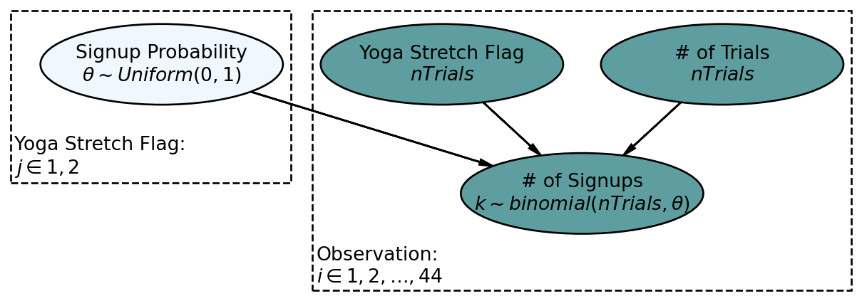
For illustration, Figure 14.3 shows the generative DAG for complete pooling. The primary assumption of this model is that each gym has the same estimated signup probabilities for with and without yoga; only two different \(\theta\) values in the entire model.
Computationally, we can go through the standard process to get our posterior.
## making a numpyro model
import numpy as np
import numpyro
import numpyro.distributions as dist
import arviz as az
from jax import random
from numpyro.infer import MCMC, NUTS

## define the graphical/statistical model as a Python function
## for posterior predictive checks, we introduce numObs argument
## which here represents len(k), the # of observations
def completePoolingModel(x, nTrials, k, numObs):
    with numpyro.plate('yogaPlate', 2):
        theta = numpyro.sample('theta', dist.Beta(concentration1=2, #alpha
                                              concentration0=2)) #beta
    ## recall yoga flag defintions
    ## p_other, p_yoga = p[0], p[1]

    with numpyro.plate('observation', numObs):
        k = numpyro.sample('k', dist.Binomial(total_count = nTrials, probs = theta[x]), obs=k)

## computationally get posterior distribution
mcmc = MCMC(NUTS(completePoolingModel), num_warmup=500, num_samples=4000)
rng_key = random.PRNGKey(seed = 111) ## so you and I get same results
mcmc.run(
    rng_key,
    x = gymDF.yogaStretch.values,
    nTrials = gymDF.nTrialCustomers.values,
    k = gymDF.nSigned.values,
    numObs = len(gymDF.nSigned.values)
) ## get representative sample of posterior
drawsDS = az.from_numpyro(mcmc).posterior ## get posterior samples into xarrayAnd ultimately we perform a posterior predictive check yielding Figure 14.4.
postSamples = mcmc.get_samples()  ##get samples for posterior pred check
from numpyro.infer import Predictive
from jax import random
rng = random.PRNGKey(seed = 111)

## Predictive is a NumPyro class used to construct posterior distributions
predictiveObject = Predictive(model = completePoolingModel,posterior_samples = postSamples)

## now make posterior predictions
## use None for data so that it gets simulated from posterior draws
postPredData = predictiveObject(
    rng_key,
    x = gymDF.yogaStretch.values,
    nTrials = gymDF.nTrialCustomers.values,
    k = None,  ### OMIT SIGNUP DATA SO IT GETS SIMULATED,
    numObs = len(gymDF.nSigned.values)
)
dataForArvizPlotting = az.from_numpyro(
    posterior = mcmc,
    posterior_predictive=postPredData
)
az.plot_ppc(dataForArvizPlotting, num_pp_samples=20, kind = "cumulative")
## mismatched bin widths is a limitation of plot_ppc(... kind = "kde"), so using cumulative instead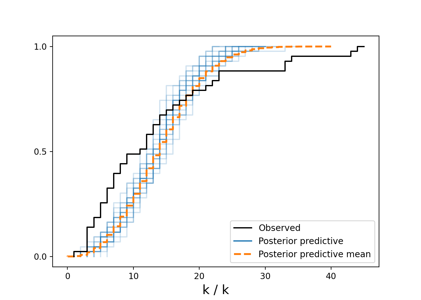
In Figure 14.4, the vertical axis represents cumulative probability. Notice that \(P(k<10)\) is much higher in the observed model than it is in the real data; this is a clue we are not capturing the essence of the generative process and the model under-predicts small observations. Similarly, notice that \(P(k>20) = 1 - P(k \leq 20)\) is also much higher in the observed model than it is in the real data; another clue, the model under-predicts large observations in addition to small ones. Successful posterior predictive checks will surround the observed data (black line in Figure 14.4) with the potential histograms from the posterior (blue lines in Figure 14.4).
14.3 No Pooling
The no pooling model treats each gym as distinct completely independent entities, i.e. the Crossfit Gym franchise has no overarching effect on success probabilities and seeing one gym’s performance offers no information for predicting another gym’s performance.
Models like this no pooling model which do not share information are ill-advised when you have small data and transferable learning like we have here. We should assume learning about one gym’s success rate should impact our opinion about another gym’s success rate - however, the model of this section cannot do that.
On our path to modelling the effects of yoga, we are going to refine our previous generative DAG to get closer to the business narrative. Specifically, we want to ensure a direct modelling of the effect of yoga stretching as an increase or decrease to the base-level, non-yoga, signup probability that exists at each gym.
Modelling this deviation directly as a linear model can lead to trouble. For example, if our model were to say “yoga increases recruitment probability by 20%”, then its possible that forecasting the effect of yoga at a gym with a base recruitment rate of 85% leads to a predicted 105% sign-up probability - this is a problem as probability of signup cannot be over 100%.
To remedy this, we use a linear predictor as input into an inverse logit link function; it ensures signup probability draws from the posterior are ALWAYS probability values between 0 and 1. This new generative story with base recruitment probability and deviation for yoga is reflected in the DAG of Figure 14.5.
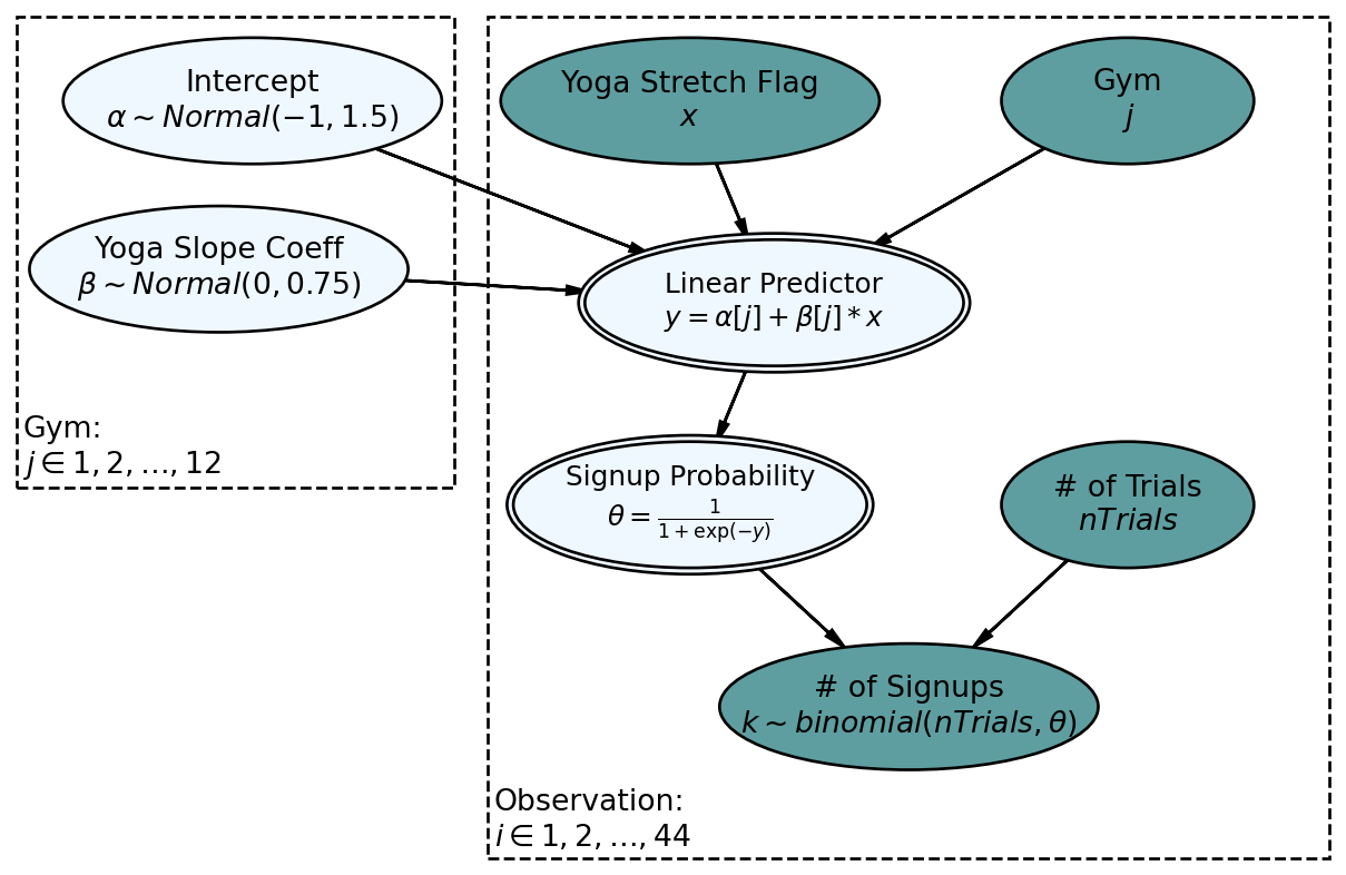
Figure 14.5 has slope and intercept terms that are not directly understandable - they go through an inverse logit function before we see their impact on a node that we can understand. To understand the prior on these terms (or any prior), simulate values and observe how they are transferred to a parameter of interest, in this case that parameter is signup probability. For now, I supply some decent priors for you.
14.3.1 Getting The Posterior Distribution
The computational model for Figure 14.5 is not simple, but all its elements have been tackled before in other chapters. Here is the code:
## making a numpyro model
from jax.scipy.special import expit as invLogit ## from JAX package, not scipy

def noPoolingModel(x, j, nTrials, k, numObs):
    with numpyro.plate('gym', len(np.unique(j))):
        alpha = numpyro.sample('alpha', dist.Normal(-1,1.5))
        beta = numpyro.sample('beta', dist.Normal(0,0.75))

    with numpyro.plate('observation', numObs):
        y = numpyro.deterministic('y', alpha[j] + beta[j] * x)
        theta = numpyro.deterministic('theta', invLogit(y))
        k = numpyro.sample('k', dist.Binomial(total_count = nTrials, probs = theta), obs=k)

## computationally get posterior distribution
mcmc = MCMC(NUTS(noPoolingModel), num_warmup=500, num_samples=4000)
rng_key = random.PRNGKey(seed = 111) ## so you and I get same results
mcmc.run(
    rng_key,
    x = gymDF.yogaStretch.values,
    j = pd.factorize(gymDF.gymID.values)[0], ## ensure compatibility with python
                                             ## zero-based indexing
    nTrials = gymDF.nTrialCustomers.values,
    k = gymDF.nSigned.values,
    numObs = len(gymDF.nSigned.values)
) ## get representative sample of posterior
drawsDS = az.from_numpyro(mcmc).posterior ## get posterior samples into xarray
## careful to restore original id's for the gyms
drawsDS = az.from_numpyro(mcmc,
coords={"gym": pd.factorize(gymDF.gymID.values)[1],
"observation": np.arange(len(gymDF.nSigned.values))},
dims={"alpha": ["gym"],
"beta": ["gym"],
"theta": ["observation"],
"y": ["observation"]}
) ## get posterior samples into xarrayWe use arviz.plot_forest() for visually inspecting the posterior estimates of our two latent variables:
az.plot_forest(drawsDS, var_names = ["alpha","beta"])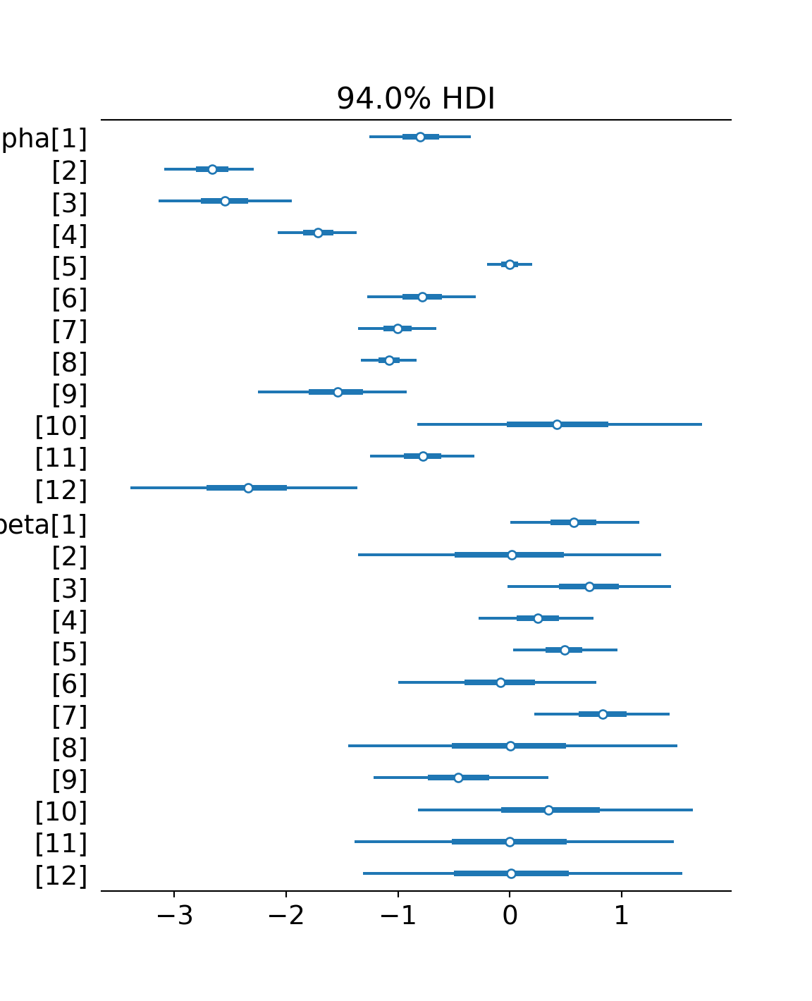
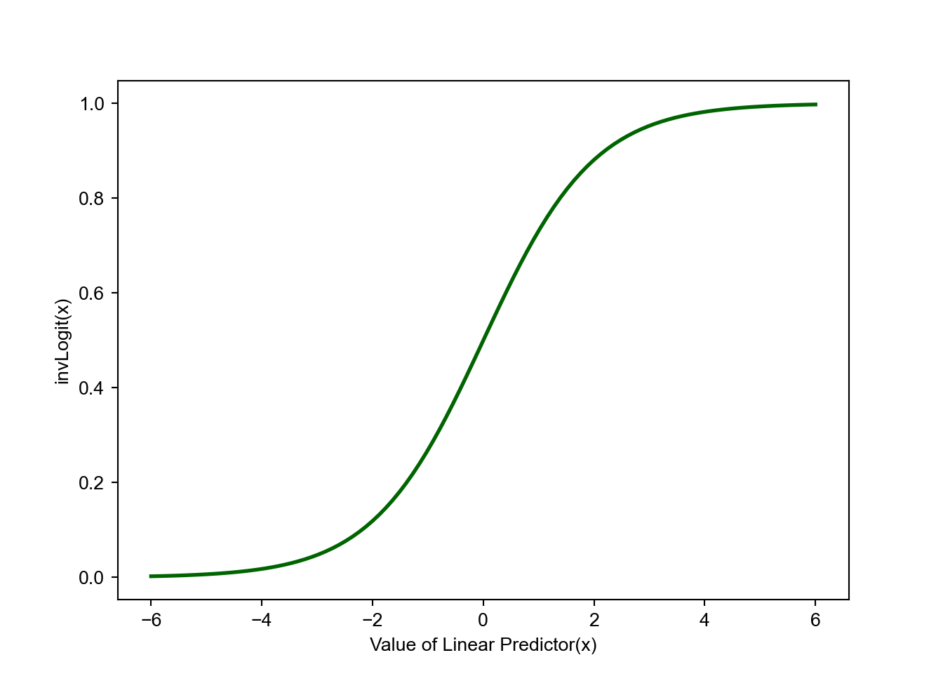
As you inspect the posterior estimates of Figure 14.6, recall that \(\alpha\) and \(\beta\) are components of a linear predictor (i.e. \(\alpha + \beta x\)). If the linear predictor is zero, that corresponds to a probability of 50% (see Figure 14.7). Hence, values for \(\alpha < 0\) would imply base conversion rates less than 50% and \(\alpha > 0\) would imply base conversion rates greater than 50%. Values for \(\beta\) indicate whether that base probability should be adjusted up or down; \(\beta < 0\) implies a negative effect for the yoga stretching routine and \(\beta > 0\) indicates that the effect is positive.
Comparing Figure 14.6 with the gym data plots of Figure 14.1, notice how the posterior estimates correspond with your expectations. The \(\alpha\) values with the smallest credible intervals are for gyms that have the largest number of trial customers participating in trials with traditional stretching (i.e. gyms 2, 5, and 8). Similarly, the \(\beta\) values with the smallest credible intervals are for gyms that have the largest number of trial customers participating in Yoga stretching classes (i.e. gyms 1 and 4). The opposite is also observable. Gyms lacking data for traditional stretching have wide credible intervals for \(\alpha\) (e.g. gym 10) and gyms lacking data for yoga stretching do not improve on the prior uncertainty in \(\beta\) (e.g. gyms 11 and 12).
This no pooling model is not terrible in the sense that each gym gets statistically modelled. Yet, Figure 14.6 reveals there are credible intervals which can be made smaller; uncertainty bands can be narrowed for gym’s missing one type of class. We know, from previous observation at all the gyms, that yoga’s effect seems small. Hence, the wide \(\beta\) uncertainty bands are not warranted. Going the other way, we should have more confidence in gym 10’s recruitment rate (\(\alpha_{10}\)). Gym 10 is a star performer and I do not think dropping the yoga-stretch will lead to enormous drops in rate. Overall, I think we should agree that learning about one gym might tell us something about another gym. In fact, I would argue that learning about 12 gym’s should tell us what we might expect when the next 100 gyms are opened. The next model explores this and shows us we can do better.
14.4 Partial Pooling
The partial pooling model imagines that the Crossfit Gyms business model produces gyms with similar characteristics. Some gyms will do better than average and some gyms will do worse, but there is some relationship between each gym’s performance. In other words, learning about one gym’s success in recruiting provides information about that gym as well as the entire population of Crossfit gyms; there is some similarity among the gyms.
To accommodate this structure (i.e. known as hierarchical or multi-level structure), we add parent nodes to the gym-level coefficients from the no pooling model. Thus, the partial pooling model generative DAG can be specified as shown in Figure 14.8.
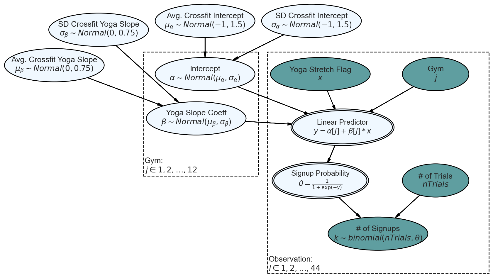
Take note of Figure 14.8’s top row of random variables characterizing the population of gyms. Think of the first two nodes as characterizing the base conversion rate for the population of crossfit gyms - one represents an expectation of any single gym’s intercept and the other represents how much deviation should be expected between the intercept’s of all the gyms. For example, a high \(\mu_{\alpha}\) and a small \(\sigma_{\alpha}\) would suggest any randomly chosen Crossfit gym will have a high base-level probability for membership sign-ups and additionally, no matter which gym is chosen, its likely to have a similarly high base-level probability.
For priors, we used our previous prior for gym-level intercept to now be the prior for its parent, \(\mu_{\alpha}\) which is the expected base intercept for any Crossfit gym. The standard deviation component, \(\sigma_{\alpha}\), uses a uniform distribution that is twice the standard deviation prior for \(\mu_{\alpha}\); chosen so the variation in base conversion rates will be on a similar scale to our own uncertainty in the corresponding mean, i.e. \(\mu_{\alpha}\).
The next two nodes atop Figure 14.8 suggest that every gym’s slope coefficient for yoga is drawn from a distribution characterized by an average effect of yoga stretching for any Crossfit gym, \(\mu_{\beta}\), and a standard deviation, \(\sigma_{\beta}\) measuring how likely any individual gym’s effect might deviate from the average. Priors are chosen as was done for the first two nodes.
Note that standard deviations of the Crossfit population parameters control how much pooling of information takes place. Larger standard deviations indicate a process where the franchise-level parameters seem to have little impact on each individual gym. Whereas, smaller standard deviations suggest that each gym has very similar characteristics.
Through these population parameters, each gym’s \(\alpha_j\) and \(\beta_j\) are related; in cases of minimal gym data, the population parameters will be very important in estimating gym performance, conversely, in cases a gym shows strong deviation from the population parameters over a lot of trial customers, then these population parameters will get ignored.
Prior distributions placed on parameters are often called hyperparameters. Feel free to just call them priors on priors if you like that better.
With generative DAG in place, we can compute and visualize the posterior in the standard way.
def partialPoolingModel(x, j, nTrials, k, numObs):
    mu_alpha = numpyro.sample('mu_alpha', dist.Normal(-1,1.5))
    sd_alpha = numpyro.sample('sd_alpha', dist.Uniform(0,3))

    mu_beta = numpyro.sample('mu_beta', dist.Normal(0,0.75))
    sd_beta = numpyro.sample('sd_beta', dist.Uniform(0,1.5))

    with numpyro.plate('gym', len(np.unique(j))):
        alpha = numpyro.sample('alpha', dist.Normal(mu_alpha,sd_alpha))
        beta = numpyro.sample('beta', dist.Normal(mu_beta,sd_beta))

    with numpyro.plate('observation', numObs):
        y = numpyro.deterministic('y', alpha[j] + beta[j] * x)
        theta = numpyro.deterministic('theta', invLogit(y))
        k = numpyro.sample('k', dist.Binomial(total_count = nTrials, probs = theta), obs=k)

## computationally get posterior distribution
mcmc = MCMC(NUTS(noPoolingModel), num_warmup=500, num_samples=4000)
rng_key = random.PRNGKey(seed = 111) ## so you and I get same results
mcmc.run(
    rng_key,
    x = gymDF.yogaStretch.values,
    j = pd.factorize(gymDF.gymID.values)[0], ## ensure compatibility with python
                                             ## zero-based indexing
    nTrials = gymDF.nTrialCustomers.values,
    k = gymDF.nSigned.values,
    numObs = len(gymDF.nSigned.values)
) ## get representative sample of posterior
## careful to restore original id's for the gyms
drawsDS2 = az.from_numpyro(mcmc,
coords={"gym": pd.factorize(gymDF.gymID.values)[1],
"observation": np.arange(len(gymDF.nSigned.values))},
dims={"alpha": ["gym"],
"beta": ["gym"],
"theta": ["observation"],
"y": ["observation"]}
) ## get posterior samples into xarrayfig, axs = plt.subplots(ncols=2, figsize=(10, 5))
# create the colors list
colors = ["purple", "grey"]
# plot the data with different colors
az.plot_forest([drawsDS2, drawsDS], var_names = "alpha", filter_vars="like", combined=True, colors=colors, ax=axs[0])
az.plot_forest([drawsDS2, drawsDS], var_names = "beta", filter_vars="like", combined=True, colors=colors, ax=axs[1])
# show the plot
plt.show()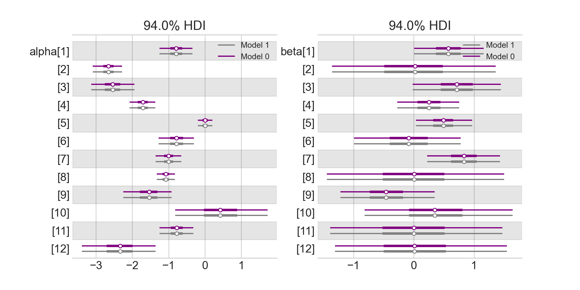
Figure 14.9 shows a slightly different snapshot of the posterior distribution. In addition to the partial pooling posterior (purple), the previous no-pooling posterior (grey) is also put on the graph for comparison. This will help us see what gains are made (or not) by adding the four hyperparameters (i.e. \(\mu_{\alpha}\),\(\mu_{\beta}\),\(\sigma_{\alpha}\),\(\sigma_{\beta}\))
Visually comparing the estimates of the two models shown in Figure Figure 14.9 helps us learn how to think about the multi-level model’s (i.e. partial pooling) interpretation:
- Uncertainty interval widths have shrunk; especially for gym/stretching combinations that are yet to be seen. For example, gym10 has only two observations, both yoga, no traditional observations. Now look at the change in \(\alpha_{10}\), the base conversion rate parameter without yoga. Its a narrower interval. The narrowness is because we have learned about the effects of yoga from the other gyms and hence, can reason better about this unobserved base rate.
- There is increased confidence that yoga stretching would be effective at each gym. Look at the rightward shift of all the partial pooling \(\beta\) estimates. Also, \(\mu_{\beta}\), the average effect of yoga is clearly greater than zero; hence, it seems like a good idea for Crossfit to promote yoga.
- Not all gym’s are equal. Looking at gym 9 where there are 3 time periods of observations - one with traditional stretching that seemed better than the others. From the partial-pooling posterior, you see a rightward shift of \(\beta_9\) as compared to the no-pooling model because we’ve learned that yoga works at other gyms. The uncertainty interval is clearly both positive and negative indicating we need more data to confidently dismiss or accept the idea of yoga.
- Both \(\alpha\) and \(\beta\) intervals in the partial pooling model often (but not always) get pulled towards their means, \(\mu_{\alpha}\) and \(\mu_{\beta}\) respectively. Because we are sharing information through these parents, their impact gets felt at the gym level - especially in cases of gym’s without much data. For example, gym 12 only has one time period of observation, so both \(\alpha_12\) and \(\beta_{12}\) intervals are pushed towards the expected values of their parent nodes. Gym 5 has a lot of data and as a result does not respond to these parental node influences.
- The interval for \(\sigma_{\alpha}\) is higher than the uniform prior belief first prescribed. Hence, this suggests that there is a lot of deviation from average expected for each new gym. Recruitment rate is quite gym-specific. We can also see this in the original data as gym 10 seems exceptional and gym 2 needs new management.
Overall, the partial pooling model is mildly helpful. Perhaps the best conclusion is drawn from \(\mu_{\beta}\) being greater than zero, yoga is helpful and that was not crystal clear when just looking at the data (Figure 14.2). More importantly, this partial-pooling model tells a coherent story about franchises and gyms that enables to craft a narrative about introducing yoga going forward.
14.4.1 Posterior Predictive Check
While these more confident and revealing estimates seem like a good thing, a posterior predictive check is in order to ensure that our model is still capable of producing data that might occasionally look like the actual data that we saw. Below is code for the posterior predictive check.
rng = random.PRNGKey(seed = 111)

## Predictive is a NumPyro class used to construct posterior distributions
predictiveObject = Predictive(model = partialPoolingModel,posterior_samples = postSamples)

## now make posterior predictions
## use None for data so that it gets simulated from posterior draws
postPredData = predictiveObject(
    rng_key,
    x = gymDF.yogaStretch.values,
    j = pd.factorize(gymDF.gymID.values)[0], ## ensure compatibility with python
                                             ## zero-based indexing
    nTrials = gymDF.nTrialCustomers.values,
    k = None,
    numObs = len(gymDF.nSigned.values)
)

dataForArvizPlotting = az.from_numpyro(
    posterior = mcmc,
    posterior_predictive=postPredData
)
az.plot_ppc(dataForArvizPlotting, num_pp_samples=20, kind = "cumulative")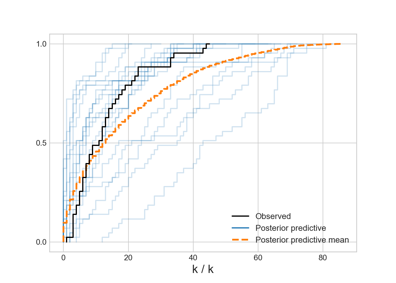
Figure 14.10 is encouraging!! It looks like the actual data might get generated from our posterior distribution. The partial pooling model seems to work! Hooray! Next chapter we interpret the results of this model for decision making.
14.5 Getting Help
TBD
14.6 Questions to Learn From
See CANVAS.